Pruning even more data with late materialization

Have you ever explored data with a quick query like the following?
‍

SELECT * FROM hits ORDER BY EventTime DESC LIMIT 10;

You want to see all columns of the first events in this table. Using SELECT * can be convenient. But loading all columns can be slow because the system needs to read a lot of data from all these columns. Consider the performance difference:

SELECT * FROM hits ORDER BY EventTime DESC LIMIT 10
WITH late_materialization_max_rows=0;
-- Execution Time: 16 s, Scanned Data: 87 GB

SELECT Title, EventTime FROM hits ORDER BY EventTime DESC LIMIT 10
WITH late_materialization_max_rows=0;
-- Execution Time 1.3 s, Scanned Data: 10 GB

The query that returns all columns scans over 8x more data and has more than 10x execution time. Note that the query turns off late materialization with late_materialization_max_rows=0.
‍

‍
Let's see what happens with late materialization:

SELECT * FROM hits ORDER BY EventTime DESC LIMIT 10;
-- Execution Time: 0.5 s, Scanned Data: 1.5 GB

This is over 30x faster than the original version and scans over 50x less data! It is even faster than selecting only the Title and EventTime columns. Since Firebolt version 4.28, this is the default behavior, so you automatically benefit from the performance improvement. You do not have to do anything to get these performance improvements.

Late materialization is not only useful for exploratory queries. The following, more complex analytical query also becomes 5x faster:

-- Without late materialization
SELECT watchid, userid, eventtime, url, title, referer,
  (responseendtiming - responsestarttiming) AS server_response_ms
FROM hits
WHERE
  eventdate BETWEEN DATE '2013-07-07' AND DATE '2013-07-14'
  AND ismobile = 1 AND responsestarttiming > 0
ORDER BY server_response_ms DESC LIMIT 10
WITH late_materialization_max_rows=0;
-- Execution Time: 1 s, Scanned Data 5 GB

-- With late materialization
SELECT watchid, userid, eventtime, url, title, referer,
  (responseendtiming - responsestarttiming) AS server_response_ms
FROM hits
WHERE
  eventdate BETWEEN DATE '2013-07-07' AND DATE '2013-07-14'
  AND ismobile = 1 AND responsestarttiming > 0
ORDER BY server_response_ms DESC LIMIT 10;
-- Execution Time: 0.2 s, Scanned Data 0.7 GB

Most data can be pruned in top-K queries

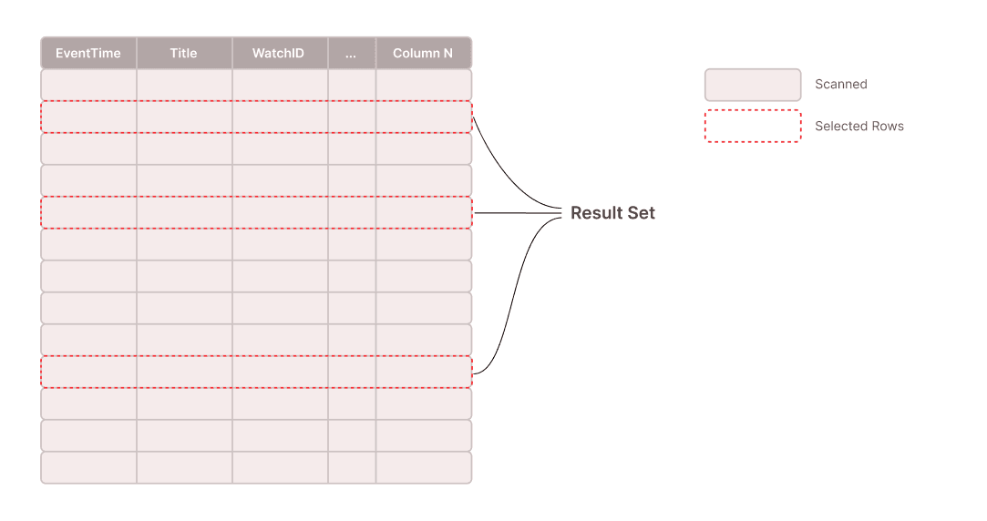
But how is it possible to reduce the amount of scanned data so drastically? The answer is simple: Most data is not actually needed to compute the result. For the queries above, only 10 rows are needed in the result. So for most columns, the system only needs to access these 10 rows, a tiny fraction of the data. Without late materialization, however, the system reads all rows just to discard most of the data.

But the system also needs to compute which 10 rows are part of the result. Fortunately, not all columns are needed to compute which rows qualify for the result. In the first example above, only the column EventTime (which has only 8 bytes per element) is needed to compute the qualifying rows. There are about 100M rows in this table. So the minimum amount of data that must be read to find the qualifying rows is about 800 MB.

Once the qualifying rows are known, the respective data from all remaining selected columns needs to be read.

How data access works in Firebolt

We previously published a blog post about data pruning in Firebolt: Making Firebolt Fast By Doing Practically Nothing. Here we repeat the most relevant points for late materialization.

Firebolt divides tables into multiple tablets. The rows in each tablet are sorted by the primary index columns. The primary index is a sparse index, so it only has entries for granules instead of individual rows. A granule is a group of 8,192 consecutive rows by default (documentation).

Tablet Pruning: Each tablet stores min-max sketches for all columns. So if you have a query of the form WHERE col_b = 10, Firebolt can check whether a tablet is guaranteed to be irrelevant to that query. For example, if the [min, max] of col_b in a tablet is [100, 200], it cannot hold the value 10 and can be pruned.

Primary Index Granule Pruning: If col_b is a column in the primary index, Firebolt can check for each granule whether it is guaranteed that no row qualifies. Note that this is slightly more difficult if the primary index has more than one column. For a primary index on (col_a, col_b), a granule with an index range of [("a", 100), ("a", 150)] can be safely pruned. A sorted range of [("a", 100), ("b", 150)], however, might contain the element ("b", 10) and cannot be ignored.

Row Lookup Pruning: A row is identified by the columns $tablet_id and $tablet_row_number in Firebolt's managed storage. If you want to scan a specific set of rows from a table, Firebolt can also perform tablet pruning and granule pruning to only scan tablets and granules that contain rows you need. This is what Firebolt uses for late materialization.

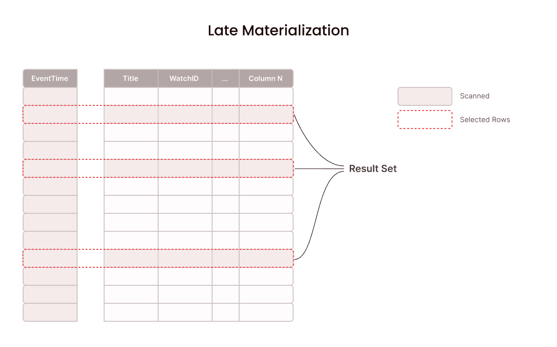
Late materialization

Late materialization is an optimization that tries to reduce the amount of scanned data as much as possible by delaying the scans of columns when possible. This optimization is made possible by storing data in a column-oriented format instead of a row-oriented format. Late materialization was researched at MIT over 18 years ago (paper) and has also recently been introduced to ClickHouse (blog post).

How late materialization is implemented in Firebolt

In Firebolt, late materialization can be expressed using query plans that leverage existing pruning techniques. When Firebolt's optimizer recognizes that it can apply late materialization it chooses a plan that loads eligible columns later. Notably, there is no new implementation for late materialization in the runtime.

The general idea is to create two scans on the same table and join them on their row ids. The first scan only provides the columns needed to compute which rows should be in the result. The second scan provides all selected columns that are not part of the first scan already. The second scan can be heavily pruned using the IDs of rows that should be in the result. After joining the result of these two scans, there is another sort to restore the order that will be changed by the join.

Here are the plans for the example query:

-- Without late materialization
EXPLAIN
SELECT * FROM hits ORDER BY EventTime DESC LIMIT 10
WITH late_materialization_max_rows=0;

[0] [Projection] hits.watchid ...
 \_[1] [Sort] OrderBy: [hits.eventtime Descending First] Limit: [10]
    \_[2] [StoredTable] Name: "hits"
          [Types]: hits.watchid ...

The plan without late materialization is rather simple. 

• [2] scans all columns of the table hits, 
• [1] sorts and limits all rows, and 
• [0] returns the result.

Now see the same query with late materialization:

-- With late materialization
EXPLAIN
SELECT * FROM hits ORDER BY EventTime DESC LIMIT 10;

[0] [Projection] hits.watchid ...
 \_[1] [Sort] OrderBy: [hits.eventtime Descending First] Limit: [10]
    \_[2] [Projection] hits.watchid ...
       \_[3] [Join] Mode: Inner [(tuple(hits.$tablet_id, hits.$tablet_row_number) = tuple(hits.$tablet_id, hits.$tablet_row_number)), (hits.$tablet_id = hits.$tablet_id), (hits.$tablet_row_number = hits.$tablet_row_number)]
          \_[4] [StoredTable] Name: "hits"
          |     [Types]: hits.watchid ...
          \_[5] [Sort] OrderBy: [hits.eventtime Descending First] Limit: [10] Relaxed Limit
             \_[6] [StoredTable] Name: "hits"
                   [Types]: hits.eventtime: timestamp not null, hits.$tablet_id: text not null, hits.$tablet_row_number: bigint not null

The plan with late materialization looks much more complicated. Here's the step-by-step breakdown: 

• [6] The first scan only includes the EventTime column and the row identifiers $tablet_id and $tablet_row_number. 
• [5]The output of this scan is sorted and limited to 10 rows. 
• [4]The second scan provides all remaining columns, but is heavily pruned by the set of row ids from [5]. This kind of pruning is also known as sideways information passing or semi join reduction. 
• [3]The scans are joined on row ids. 
• [2]Removes row id columns which are no longer needed. 
• [1]Sort because the join can change the sort order from [5]. 
• [0]The result is returned.

If you wonder whether your query already uses late materialization, you can check the EXPLAIN output of your query for this self join pattern. You can also manually control whether late materialization should be used if you want to override Firebolt's optimizer.

How you can control late materialization in Firebolt

Firebolt only applies late materialization for queries with a limit of 10 or smaller by default. If you choose a limit higher than that, you will observe that late materialization will not be triggered anymore:

SELECT * FROM hits ORDER BY EventTime DESC LIMIT 100;
-- Execution Time: 16 s, Scanned Data: 87 GB

If you want to override this decision and apply late materialization anyway, you can use the late_materialization_max_rows system setting:

SELECT * FROM hits ORDER BY EventTime DESC LIMIT 100
WITH late_materialization_max_rows=100;
-- Execution Time: 0.8 s, Scanned Data: 2 GB

You can either set this setting per query using the WITH clause as outlined in the example above or apply it to the whole session using a SET statement:

SET late_materialization_max_rows=100;
SELECT * FROM hits ORDER BY EventTime DESC LIMIT 100;
-- Execution Time: 0.8 s, Scanned Data: 2 GB

If you want to turn it off completely, you can set the value to 0:

SELECT * FROM hits ORDER BY EventTime DESC LIMIT 10
WITH late_materialization_max_rows=0;
-- Execution Time: 16 s, Scanned Data: 87 GB

When should you use late materialization?

Why should you ever want to turn late materialization off? Because it is not equally effective in all cases. There are two main properties a query needs to have to benefit from late materialization:

• Column Size: The larger the byte size of the columns that are loaded late, the larger the improvement from late materialization. If there is a huge string column where each element is thousands of characters long on average, it will be much faster to only load parts of this data using effective pruning. In contrast, if all your strings are only one character long, there is not much to gain.

• Row Count Difference: Late materialization is only effective if it can prune data better than a regular scan. If your table has only 10 rows, you don't need late materialization. Note that Firebolt also pushes filters into the scan and prunes reads using these filters. If only 10 rows are returned from the scan, there is nothing to gain from applying late materialization. However, if the scan returns millions of rows, there is a lot to gain.

Running a more complex query plan with two scans and a join adds a small overhead in execution time. Whether late materialization is beneficial to a query depends on whether it prunes enough data to make up for this overhead. For some queries, this easily pays off and results in immense speedups. Other queries might not benefit at all and can even get a few milliseconds slower. This is why Firebolt applies late materialization only for limits of 10 and smaller by default, a very conservative threshold.

An ideal use case

Here's another example where late materialization offers tremendous benefits. In this use case the session table contains a history of API requests for a cloud service. Say you are interested in investigating the requests with the worst response time on a specific day:

-- Without late materialization
SELECT read_bytes, query_telemetry
FROM query_history_f
WHERE query_start_date = '2025-09-01'
ORDER BY read_bytes DESC LIMIT 10
WITH late_materialization_max_rows = 0;
-- Execution Time: 11 s, Scanned Data: 75 GB

-- With late materialization
SELECT read_bytes, query_telemetry
FROM query_history_f
WHERE query_start_date = '2025-09-01'
ORDER BY read_bytes DESC LIMIT 10
WITH late_materialization_max_rows = 10;
-- Execution Time: 0.2 s, Scanned Data: 0.2 GB

A very useful column is query_telemetry, which stores execution statistics in a JSON format. Elements in this column are usually very large. Also, there are many queries every day. Consequently, column size and row count difference are very large, and this query benefits strongly from late materialization.

Now, see examples where late materialization does not help:

Too small columns

-- Without late materialization
SELECT UserAgentMinor
FROM hits
ORDER BY EventTime LIMIT 10
WITH late_materialization_max_rows=0;
-- Execution Time: 0.4 s, Scanned Data: 1.9 GB

-- With late materialization
SELECT UserAgentMinor
FROM hits
ORDER BY EventTime LIMIT 10;
-- Execution Time: 0.4 s, Scanned Data: 1.5 GB

UserAgentMinor is a very short string column. There are usually only two characters per element. This is so little data that late materialization just does not pay off. Even though the version with late materialization scans a tiny bit less data, the execution time is equal for both versions.

Too little difference in row counts

-- Without late materialization
SELECT *
FROM hits
WHERE EventTime <= '2013-07-01 20:00:00'
ORDER BY EventTime LIMIT 10
WITH late_materialization_max_rows=0;
-- Execution Time: 0.5 s, Scanned Data: 0.9 GB

-- With late materialization
SELECT *
FROM hits
WHERE EventTime <= '2013-07-01 20:00:00'
ORDER BY EventTime LIMIT 10;
-- Execution Time: 0.4 s, Scanned Data: 1.5 GB

Here you have an extremely selective filter. Only 39 elements have an event time that is as early as 2013-07-01 20:00:00. The row count difference is too small. Here you can also see that late materialization pruning is not perfect. The version with late materialization scans a little more data than the version with a single scan that prunes with the filter predicate.

Conclusion

Late materialization is an optimization that can offer tremendous speedups for top-K queries by reducing the amount of data that needs to be scanned. In Firebolt, you benefit from it automatically.

This blog post described the opportunity to prune data in top-K queries and how Firebolt uses it with late materialization. It explained how late materialization is implemented in Firebolt and how you can see it in the query plan. Finally, it showed in which cases late materialization can improve performance and when it doesn't help.

If you want to know more, check out the documentation on late materialization or get started with Firebolt yourself.