TL;DR

This post describes different methods for reducing the number of scanned rows in a query (a.k.a. pruning), which improves query performance. From these methods, the post chooses to focus on sketch-based row pruning, its benefits, and how it’s represented in Firebolt.

Introduction

A famous saying in the world of low-level development is "The key to making programs fast is to make them do practically nothing". Unsurprisingly, this is also true for SQL databases. During the planning phase, Firebolt tries different optimizations in order to make a query plan more efficient. An inefficient plan usually involves doing the same work many more times then we have to. For example, the plan may run a scalar operation on 1B values, even though we’re going to discard them later. One such optimization to avoid doing unnecessary work is row pruning.

To discuss why it matters, let's say that for an online game, we have a table players with 30 columns, on which we run the following query:

SELECT id
FROM players
WHERE hours > 10000 AND country = 'Laputa';

Since Firebolt is already a columnar database, we only read the data for the columns id, country, and hours from storage, avoiding all other columns. However, let’s say that only 0.1% of our playerbase are Laputans. Furthermore, let’s say that due to legal issues, the game was only introduced to the people of Laputa 450 days ago. Since there’s only 24 hours in a day, a player that has more than 10,000 hours had to play it for at least 416 days, meaning that only the players who bought the game in the first 34 days after it was published, about 20% of all Laputan players, are eligible, reducing the 0.1% into 0.02%.

If we don’t use any of this knowledge, then we are going to end up reading the data for all players and then use only a 5000th of it. For queries as computationally simple as this, where most of the time spent by the query is spent on I/O, reading all that data would be a major bottleneck that we’d like to avoid. It is for this reason that row pruning is crucial.

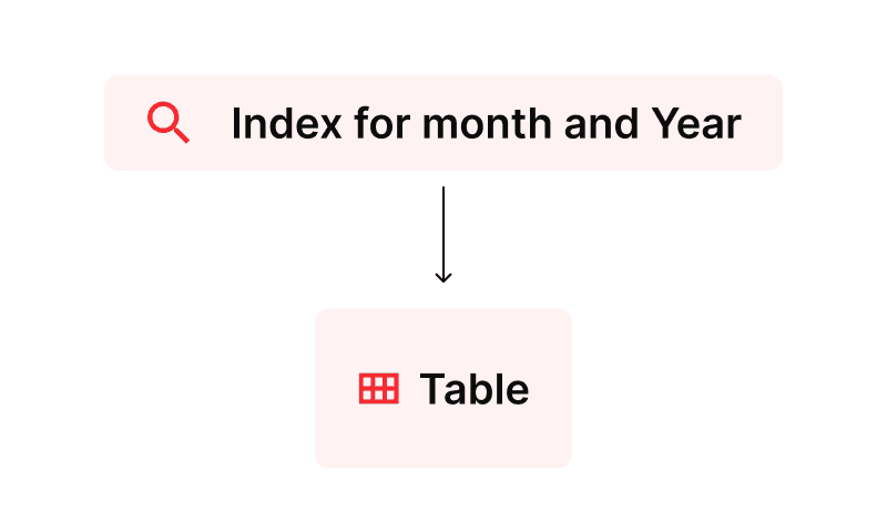
What is row pruning?

Just as column pruning allows the database to avoid reading columns that are not required for evaluating the query, row pruning refers to every optimization that allows the database to avoid reading rows that are not required for evaluating the query. Some commonly used forms of row pruning are:

• Secondary indexes - For a specific expression, a data structure is constructed during insertion that allows the database to quickly retrieve, for every X, the list of rows for which the expression is less/more/equal to X. B-trees allow retrieving this information with at most O(log(n) + k) reads from disk, where n is the total number of rows in the table, and k is the number of rows satisfying the search criteria.
  

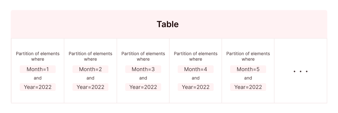
• Partitions - For a specific expression, the table is internally divided into subtables where, for each row in a subtable, all values of the expression are the same. 

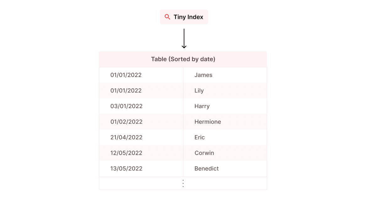
• Clustering indexes - The table itself is sorted by the index expression, and the index data structure now indexes ranges (named “granules”) within the table instead of individual rows. As the index data structure now indexes fewer things, it can become small enough to fit entirely in RAM.
  

Firebolt supports both partitions and clustering indexes. Yet, both of these methods present two problems:

• The database administrator (DBA) must explicitly decide which column(s) will be used for partitioning/indexing.
• Unless we’re willing to create several copies of the table, only one set of column(s) can be used for partitioning/indexing (note that B-tree based secondary indexes do not suffer from this limitation).

If we look at our original example, the query’s WHERE clause checked two fields: hours and country. Unless usage of queries on these fields is very frequent, it is very unlikely that the DBA would use them as an index/partition, since using these fields prevents them from picking other fields, which might be used in much more frequent queries. As we’ve mentioned above, this specific query is also very correlated with the date when the player registered in the game. However, taking advantage of this correlation requires a planner smart enough to deduce it, which isn’t trivial.

In order to overcome these problems, Firebolt uses a fourth type of pruning: sketch-based row pruning.

What is sketch-based row pruning?

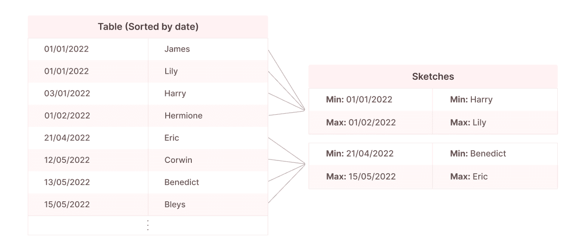
All pruning methods described above require special preparation during INSERT: splitting the data into partitions, sorting the data, or building an index structure. Sketch-based row pruning is similar to indexing, but instead of a full index, we only build small, per-tablet sketches. Unlike an index, a sketch can be built separately and cheaply for every column. A sketch contains statistical properties of the column values. Some possible properties that a sketch can contain are:

• A boolean signifying whether the column contains NULL values
• A set of all occurring values for the column.
• A Bloom filter‍
• A binned histogram
• Lower and upper bounds

Firebolt sketches only support lower and upper bounds at the moment. So, as an example:

‍

Since sketches are created for every column, there’s no need for the DBA to choose specific columns for sketches. Now let’s go back to the players table. 

SELECT id
FROM players
WHERE hours > 10000 AND country = 'Laputa';

As mentioned earlier, the players we are looking for registered in the game during the first 34 days after it launched. Under the reasonable assumption that players are added to the database roughly at the same time they registered, it is likely that these players would be stored within a small set of tablets that was added around those 34 days. This means that for all tablets created later, the hours field will always be less than 10000, which would show in a lower-upper bounds sketch, allowing us to discard them without reading their contents. 

Furthermore, if our sketches support Bloom filters (or even just a set of all possible values, as there are only 195 countries in the world), we can also get rid of all the tablets that were added before our game launched in the country of Laputa. 

This example shows how sketches can implicitly capture correlations between table columns and their insertion time, without these having to be specified explicitly by the DBA. Furthermore, sketches can also help us with equality predicates against very rare predicates. If we store a sketch of unique country values for every 1000 rows, then since only 0.02% of players are Laputans (every 5000th player), we can avoid scanning almost 80% of rows, as most blocks of 1000 rows won't contain a Laputan and can be pruned.

A real life use case

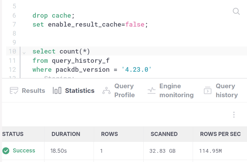
One of the tables we commonly use in internal Firebolt processes is called query_history_f. This table, along with several others, keeps a history of the queries that ran on our Firebolt cloud. Let’s say that we are interested in getting information about queries that ran on a specific version of Firebolt that had some unique behavior. In this case, we would use the query_history_f.packdb_version field to filter on these queries. For simplicity’s sake, let's say we only want to count them, which means that our query would be the following:

SELECT count(*)
FROM query_history_f
WHERE packdb_version = '4.23.0';

Below, we can see what happens when we run this query with and without using sketch based row pruning.

Without sketch-based row pruning:

With sketch-based row pruning:

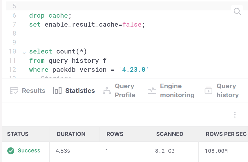
Let us now also take a look at the EXPLAIN (ANALYZE) output for the query with and without sketch-based row pruning. Both EXPLAIN outputs have the read_tablets table function, and we can see that without sketch-based row pruning, it had to read 2,126,392,391 rows, and with sketch-based row pruning it only read 522,026,101 rows. If we look at the list_tablets table function, we can similarly see that both versions read a nearly identical number of tablets (~1110). The difference between both versions happens between list_tablets and read_tablets. In the version without sketch-based row pruning, they appear on top of each other, while in the version with sketch-based row pruning, there’s a [Filter] between them which cuts the ~1110 tablets into only 92. In the next two sections, we’re going to explain why we choose this specific representation for sketch-based row pruning.

Without sketch-based row pruning:

[0] [Projection] ref_0
|   [RowType]: bigint not null
|   [Execution Metrics]: Optimized out
 \_[1] [Aggregate] GroupBy: [] Aggregates: [count(*)]
   |   [RowType]: bigint not null
   |   [Execution Metrics]: output cardinality = 1, thread time = 1ms, cpu time = 1ms
    \_[2] [Projection]
      |   [RowType]: 
      |   [Execution Metrics]: output cardinality = 5512650, thread time = 0ms, cpu time = 0ms
       \_[3] [Filter] (ref_0 = '4.23.0')
         |   [RowType]: text null
         |   [Execution Metrics]: output cardinality = 5512650, thread time = 6236ms, cpu time = 6175ms
          \_[4] [TableFuncScan] $0.packdb_version
            |   $0 = read_tablets(table_name => query_history_f, ref_0)
            |   [RowType]: text null
            |   [Execution Metrics]: output cardinality = 2126392391, thread time = 29451ms, cpu time = 17721ms
             \_[5] [TableFuncScan] $0.tablet
               |   $0 = list_tablets(table_name => query_history_f)
               |   [RowType]: tablet not null
               |   [Execution Metrics]: output cardinality = 1113, thread time = 8ms, cpu time = 7ms
                \_[6] [Projection]
                  |   [RowType]: 
                  |   [Execution Metrics]: output cardinality = 0, thread time = 0ms, cpu time = 0ms
                   \_[7] [SystemOneTable]
                         [RowType]: integer not null
                         [Execution Metrics]: Nothing was executed

With sketch-based row pruning:

[0] [Projection] ref_0
|   [RowType]: bigint not null
|   [Execution Metrics]: Optimized out
 \_[1] [Aggregate] GroupBy: [] Aggregates: [count(*)]
   |   [RowType]: bigint not null
   |   [Execution Metrics]: output cardinality = 1, thread time = 1ms, cpu time = 1ms
    \_[2] [Projection]
      |   [RowType]: 
      |   [Execution Metrics]: output cardinality = 5512650, thread time = 0ms, cpu time = 0ms
       \_[3] [Filter] (ref_0 = '4.23.0')
         |   [RowType]: text null
         |   [Execution Metrics]: output cardinality = 5512650, thread time = 1256ms, cpu time = 1240ms
          \_[4] [TableFuncScan] $0.packdb_version
            |   $0 = read_tablets(table_name => query_history_f, ref_0)
            |   [RowType]: text null
            |   [Execution Metrics]: output cardinality = 522026101, thread time = 5891ms, cpu time = 4296ms
             \_[5] [Projection] ref_0
               |   [RowType]: tablet not null
               |   [Execution Metrics]: Optimized out
                \_[6] [Filter] (((ref_1 > '4.23.0') or (ref_2 < '4.23.0')) IS DISTINCT FROM TRUE)
                  |   [RowType]: tablet not null, text null, text null
                  |   [Execution Metrics]: output cardinality = 92, thread time = 42ms, cpu time = 39ms
                   \_[7] [TableFuncScan] $0.tablet, $0.min_packdb_version, $0.max_packdb_version
                     |   $0 = list_tablets(table_name => query_history_f)
                     |   [RowType]: tablet not null, text null, text null
                     |   [Execution Metrics]: output cardinality = 1110, thread time = 47ms, cpu time = 14ms
                      \_[8] [Projection]
                        |   [RowType]: 
                        |   [Execution Metrics]: output cardinality = 0, thread time = 0ms, cpu time = 0ms
                         \_[9] [SystemOneTable]
                               [RowType]: integer not null
                               [Execution Metrics]: Nothing was executed

The classical representation of sketch-based row pruning

These two last sections will be dedicated to explaining how we represent sketch based row pruning in our system. Let’s take the original example of our players table, but simplify the query to also include non-Laputans. The new, simpler query is now:

SELECT id
FROM players
WHERE hours > 10000;

What this query needs to do is, for every tablet, look at its bounds and determine whether its upper bound is less than or equal to 10000. If it is, then we can skip that tablet when running the query. Now that we know how we want to execute the query, one question remains: how can we express this behavior in the query plan?

A naive query plan without sketch-based row pruning would look roughly like this (sadly we can’t bring an actual Firebolt example here, as Firebolt no longer uses this representation):

Project id
    Filter hours > 10000
        ReadFromStorage players.hours, players.id

Query plans are trees executed from bottom-to-top, meaning that this query plan represents the following steps: read the columns from storage, then filter them, then return the id to the user. Now, let’s represent our sketch based row pruning in the most obvious way:

Project f2
    Filter f1 > 5
        ReadFromStorage t.f1, t.f2, WithPruning t.f1 > 5

While this looks very easy to read, it also has some problems. 

• First of all, we have made the semantics of ReadFromStorage more complicated since it can now accept an optional WithPruning clause. 
• More than that, WithPruning accepts an expression. Is any arbitrary boolean returning expression allowed in WithPruning? If that's not the case, then we need to define the exact semantics of what expressions WithPruning accepts. 
• WithPruning hides the actual runtime behavior from us. Filter or Project or ReadFromStorage can be easily explained, but what does WithPruning actually cause the runtime to do? The runtime has to interpret the expression and then decide how to use the sketch to prune, creating a “planner-within-runtime” situation.
• If we ever support reading from different types of storage, or from table functions, do we also want these to support WithPruning? In that case, we would have to ensure each of these table source nodes allows such a clause.

The last point is especially important for us, as we want to support reading from different data sources and not just from our managed tables. Firebolt also supports reading from an Iceberg lakehouse, where we'd like all our optimizations to work just as well. The good news is that Iceberg can also provide a lower-upper-bound sketch for its tablets. But does this mean that we should reimplement WithPruning for a ReadFromIceberg node? Should we have a hidden layer within Firebolt code that generalizes ReadFromStorage and ReadFromIceberg so that both can handle WithPruning the same? 

Composable pruning

What we really want is to be able to express WithPruning as its own node in the query plan, to decouple it from ReadFromStorage. This would make it less opaque, as well as allow it to easily compose together with ReadFromIceberg or any other ReadFromXXX. Such a composable approach is described in the paper “Big Metadata: When Metadata is Big Data.” The main idea here is to separate ReadFromStorage into two primitives: ListTablets, ReadTablets. ReadTablets will not be a table source node, as that role will be reserved for ListTablets. The old ReadFromStorage can now be replaced with a ReadTablets on top of a ListTablets. Here is an EXPLAIN (PHYSICAL) for such a query (note that there’s still no pruning here): 

[0] [Projection] players.id
 \_[1] [Filter] (players.hours > 10000)
    \_[2] [TableFuncScan] players.id: $0.id, players.hours: $0.hours
      |   $0 = read_tablets(table_name => players, tablet)
      |   [Types]: players.id: bigint null, players.hours: integer null
       \_[3] [TableFuncScan] tablet: $0.tablet
         |   $0 = list_tablets(table_name => players)
         |   [Types]: tablet: tablet not null
          \_[4] [Projection]
             \_[5] [SystemOneTable]
                   [Types]: $0: integer not null

Note that in our implementation, ReadTablets and ListTablets have become table-valued functions (and are also named using snake_case instead). list_tablets returns a "metatable" containing the list of tablet "paths" for the players table and metadata for each tablet. read_tablets can no longer decide what it reads on its own, so it has to instead accept input from list_tablets which contains the "paths" for the tablets it will read. By using this representation, we have managed to formalize the separation between "read from storage" and "decide what to read" into the query plan itself. 

The next step would be to express the pruning of blocks using metadata. Since list_tablets returns a list of tablet "paths" and their metadata, we can use said metadata, which would include the sketch, to filter out only the tablets that we want. Doing this will get us the following query plan, where in addition to the obvious [Filter] on hours, we also have a [Filter] on tablet metadata that runs before we even start reading the tablets:

[0] [Projection] players.id
 \_[1] [Filter] (players.hours > 10000)
    \_[2] [TableFuncScan] players.id: $0.id, players.hours: $0.hours
      |   $0 = read_tablets(table_name => players, tablet)
      |   [Types]: players.id: bigint null, players.hours: integer null
       \_[3] [Projection] tablet
          \_[4] [Filter] ((max_hours <= 10000) IS DISTINCT FROM TRUE)
             \_[5] [TableFuncScan] tablet: $0.tablet, max_hours: $0.max_hours
               |   $0 = list_tablets(table_name => players)
               |   [Types]: tablet: tablet not null, max_hours: integer null
                \_[6] [Projection]
                   \_[7] [SystemOneTable]
                         [Types]: $0: integer not null

We no longer have a special WithPruning clause or even a new node representing pruning. Instead, the pruning operation is simply a standard SQL filter done on standard SQL fields, which just happen to be the same fields we will later use to read players. Note that IS DISTINCT FROM TRUE is used in order to allow a sketch to be NULL for backward compatibility with storage where it was not yet calculated. 

Finally, as mentioned earlier, using this we can also easily represent such pruning on Iceberg. For example, the query

SELECT l_linenumber
FROM read_iceberg('s3://firebolt-core-us-east-1/test_data/tpch/iceberg/tpch.db/lineitem')
WHERE l_receiptdate > '2001-01-01';

gets the following EXPLAIN (PHYSICAL) (where some field names have been replaced with ... to make the plan more easily readable):

[0] [Projection] l_linenumber
 \_[1] [Filter] (l_receiptdate > DATE '2001-01-01')
    \_[2] [TableFuncScan] l_linenumber: $0.l_linenumber, l_receiptdate: $0.l_receiptdate
      |   $0 = read_from_s3(url='s3://firebolt-core-us-east-1/test_data/tpch/iceberg/tpch.db/', format='PARQUET', object_pattern='*', type=Iceberg, file_format, file_size, ...)
      |   [Types]: l_linenumber: bigint null, l_receiptdate: date null
       \_[3] [Filter] ((max_l_receiptdate <= DATE '2001-01-01') IS DISTINCT FROM TRUE)
          \_[4] [MaybeCache]
             \_[5] [TableFuncScan] ...
               |   $0 = list_iceberg_files(url => 's3://firebolt-core-us-east-1/test_data/tpch/iceberg/tpch.db/lineitem/metadata/00001-8e0eaefb-ab69-4db0-99ea-8fe78f974ab7.metadata.json', metadata_json_content => '****', snapshot_id => '...', snapshot_timestamp => NULL)
               |   [Types]: file_format: ...
                \_[6] [Projection]
                   \_[7] [SystemOneTable]
                         [Types]: $0: integer not null

Using this approach, we’ve managed to add support for sketch-based row pruning on Iceberg without having to write any specialized pruning code, relying only on our already-existing pruning infrastructure and on reading Iceberg metadata.

Conclusion

In this post, we have shown the benefits and implementation of lower-upper-bound sketch-based row pruning. We can also extend what a sketch can contain and use composable pruning to allow for some more useful optimizations down the line:

• Firebolt’s join pruning currently uses only the clustering index. It can be extended to take advantage of sketches as well by adding matching Filters on top of ListTablets.
• Pruning on WHERE x > (SELECT max(y) FROM t) becomes much easier to implement. This can be done by adding the subquery into our existing Filter node on top of ListTablets.
• Queries with a LIMIT on top of a Filter can use a Sort on top of ListTablets to sort tablets in descending order according to how many rows are estimated to survive filtering, allowing the query to finish earlier.