Technical Deep Dive: Efficient and ACID Compliant Vector Search Indexes in Firebolt

Introduction

Modern AI applications heavily rely on semantic search through embeddings: High-dimensional numerical vectors that represent entities such as text, images, and audio. Efficiently searching these embeddings for the "top K closest points" in a multi-dimensional vector space, known as vector search or similarity search, is crucial. This deep dive explores how Firebolt implements native vector search indexing and search capabilities to enable these demanding AI workloads.

The Need for Vector Search in Firebolt

For a long time, most of the vector search use cases powered by Firebolt involved moderately sized datasets, on the order of a few million embeddings. In these scenarios, computing exact distances between the query’s target vector and all stored embeddings through a full table scan was both simple and fast enough. There was no pressing need for specialized indexing or approximate methods.

That changed when the Similarweb team brought us a very different challenge. Their workload involved running a semantic similarity search over a table containing hundreds of millions of embeddings. For them, query latencies of 20–30 seconds with brute-force nearest neighbor search were unacceptable. They needed sub-second search times to support interactive, production-grade applications, which is exactly what Firebolt is built for.

This is precisely the kind of scenario that traditional full-scan approaches cannot handle efficiently. At this scale, computing exact distances for every query quickly becomes prohibitively expensive. To meet these new requirements, Firebolt introduced native vector search indexing based on Approximate Nearest Neighbor (ANN) techniques, using the Hierarchical Navigable Small World (HNSW) graph technique. ANN methods trade ingest performance and a small amount of accuracy for dramatically improved lookup performance, a trade-off that is often more than acceptable in real-world, analytical AI applications.

With Firebolt’s vector search indexes, Similarweb was able to improve their production performance by 100x, reducing query execution times from tens of seconds to around 300 ms (99th percentile), enabling fast and scalable semantic search on massive datasets, all within the same compute cluster that powers their analytical workloads.

How Vector Search Indexes Are Used in Firebolt

For a full rundown of how to use vector search indexes in Firebolt, see our documentation. Here’s an example usage that we will use throughout this blog post.

Let’s assume we have a table documents that stores embeddings as an array of real numbers as well as some id for these embeddings:

CREATE TABLE documents
 (id int, embedding array(real not null) not null);

We can now create a vector search index using HNSW for these 256-dimension embeddings with the following query:

CREATE INDEX documents_vec_index
ON documents
USING HNSW ( embedding vector_cosine_ops )
WITH ( dimension = 256 );

Assuming the embeddings were generated using the AWS Bedrock amazon.titan-embed-text-v2:0 model, we can now search for the 10 documents that are semantically most similar to the search term “low latency analytics” using the vector_search table-valued function like this:

SELECT
  *
FROM
  vector_search (
    INDEX documents_vec_index,
    target_vector => (
      SELECT
        AI_EMBED_TEXT (
          MODEL => 'amazon.titan-embed-text-v2:0',
          INPUT_TEXT => 'low latency analytics',
          LOCATION => 'bedrock_location_object',
          DIMENSION => 256
        )
    ),
    top_k => 10
  );

We are using the AI_EMBED_TEXT function to obtain a vector embedding for our search term in this example, but you could also get it using any other subquery on your database or simply pass it in as a constant value. The result of the vector_search table-valued function is (at most) top_k rows with the same columns as the original documents table. So the query above will return columns id and embedding.

High-Level Architecture

Let’s have a look at how vector search indexes are implemented in Firebolt at a high level. Each tablet within Firebolt maintains its own dedicated vector index file for every vector search index defined on the table, this makes the indexes fully transactional and ACID compliant. These files each represent an HNSW index created using the USearch library. For every vector, Firebolt stores the row number of the corresponding row in the tablet inside the USearch index. This association between the vector’s position in the index and its row number, together with the tablet identifier, provides a precise mapping from entries in the vector index files back to the actual table rows.

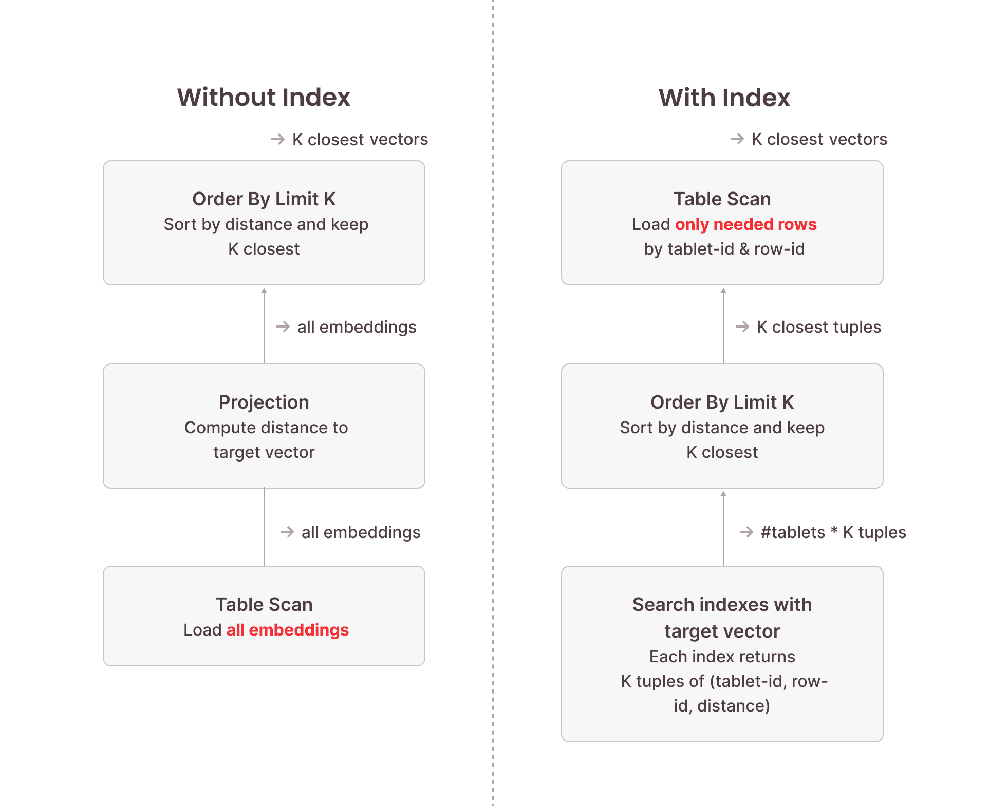
When a vector search query is executed, Firebolt initiates searches across each tablet's vector index file using USearch. This process identifies the relevant row numbers corresponding to the closest vectors. More precisely, when searching for the top K closest vectors to a target vector, this will return up to K results per tablet. So we need to condense this down to the overall top K closest vectors using an ORDER BY … LIMIT K operator in the execution pipeline. Once these row numbers are obtained, Firebolt performs an optimized base-table scan of these rows. Critically, this scan is not a full table scan; instead, it selectively reads only the rows identified by the vector index, significantly reducing the amount of data processed.

The following image illustrates the difference between vector search using a vector search index and brute-force vector search without an index. Because the index structure is optimized for this specific task and doesn’t need to inspect each vector stored in the index, searching the vector search indexes is orders of magnitude faster than a full table scan. The table scan performed afterwards only needs to load a fraction of the data stored in the table because we know their precise location from the vector index.

Caching and In-Memory Processing of Vector Search Indexes

With the architectural foundations in place, let’s look at some of the performance characteristics of these indexes and how Firebolt manages them at runtime.

The performance of vector search depends not just on the algorithm, but also on how efficiently the system can access the index structure. Firebolt’s vector search indexes are built using the USearch library, which is optimized for in-memory access. By default, Firebolt loads the full vector index files into memory when they are first queried and keeps them cached for subsequent searches. This strategy, controlled via the load_strategy = in_memory setting, delivers the best possible query latency once loaded: lookups happen entirely in RAM, and subsequent vector searches avoid any disk I/O overhead. Firebolt Compute Clusters that have enough memory to hold all relevant indexes can achieve highly predictable and consistently low latencies.

However, not all workloads or compute cluster configurations allow indexes to remain resident in memory. For those with tighter memory budgets, Firebolt supports a disk-backed mode via load_strategy = disk. In this mode, index files are memory-mapped, which means the operating system decides when pages are loaded into memory and when they are evicted. This significantly reduces memory requirements, but at a cost: if a needed portion of the index is not available as a mapped in-memory page, it must be read from SSD again. As a result, queries may exhibit higher latency and less predictable performance compared to fully in-memory operations. This can happen for both recurring target vectors (the pages could have been evicted) and never-before-seen target vectors (part of the index structure has never been loaded)

In practice, users often choose the strategy based on workload characteristics. Latency-sensitive or high-throughput workloads typically run on compute clusters sized to keep all indexes in memory, ensuring optimal speed. Less critical or exploratory workloads can trade off some performance for cost efficiency by using disk-backed mode. The section on Best Practices for High-Performance Vector Indexing explains how to monitor cache behavior and configure Firebolt accordingly.

Maintaining Vector Search Indexes: ACID Compliance and Speed

Some systems, including specialized vector databases, trade off transactional guarantees to simplify index maintenance, which can lead to inconsistencies between the data and the index. Firebolt takes a different approach: vector search indexes are fully ACID-compliant and transactionally consistent with the underlying table data. This ensures that searches always reflect the exact state of the database at the time of the query, even under concurrent writes or failures.

A key element of this design is Firebolt’s tablet-based storage model. Inserts always create new tablets, and each tablet has its own corresponding vector index file. When data is inserted, Firebolt builds the vector index for the new tablet as part of the same transaction that writes the base table data. Once the transaction commits, the new data and its index appear together in the same snapshot. Deletes are handled through a separate per-tablet delete file. Vector search operations transparently consult this file to exclude deleted rows, maintaining correct results without requiring index rebuilds.

When ingesting data in bulk, Firebolt first writes the incoming data into intermediate tablets. These tablets are then merged into larger, finalized tablets before being uploaded to cloud storage and committed. Vector indexes are only built for the finalized tablets, which avoids the overhead of repeatedly building indexes on temporary intermediates while still preserving full transactional consistency.

In some cases, tablets may exist without an associated vector index file, for example, when an index is created after data has already been inserted. When this happens, users can bring the table fully up to date by running VACUUM (REINDEX=TRUE), which identifies any tablets without vector index files and builds the missing index files. This operation is fully transactional: it integrates cleanly with concurrent workloads and ensures that the index state always corresponds exactly to a well-defined snapshot of the table. For an explanation of how Firebolt handles tablets without index files during searches, see the section on handling unindexed tablets.

Firebolt’s internal bookkeeping ensures that the presence or absence of index files is always tracked precisely. Queries run against a coherent view of which tablets are indexed and which are not, even as data is inserted, deleted, merged, or reindexed in parallel. As a result, the system consistently returns correct results and maintains strong transactional semantics, without requiring users to manage index consistency manually or forfeit data consistency.

Best Practices for High-Performance Vector Indexing

Getting the best out of Firebolt’s vector search indexes comes down to two main aspects: making sure the index files fit in memory, and structuring the table in a way that minimizes the amount of data scanned after the index lookup.

The first step is to ensure that your engine has enough memory to keep the vector index files fully in memory. You can check the size of each index through the uncompressed_bytes column in information_schema.indexes:

SELECT index_name, uncompressed_bytes, number_of_tablets
FROM information_schema.indexes
WHERE table_name = 'documents' and index_type = 'vector_search';

Compare the reported index sizes with the defined cache size limit for vector search indexes.

SELECT sum(pool_size_limit_bytes) AS vector_index_cache_size_bytes
FROM information_schema.engine_caches
WHERE pool = 'vector_index' and cluster_ordinal = 1;

Firebolt lets you configure how much of that memory should be used for caching vector index files using the engine-level VECTOR_INDEX_CACHE_MEMORY_FRACTION configuration:

ALTER ENGINE my_engine
SET VECTOR_INDEX_CACHE_MEMORY_FRACTION = 0.6; 
-- up to 60% of the each node's memory can be used for caching vector search indexes

If an index is too large to fit into memory after appropriate engine sizing, the next lever to consider is adjusting the HNSW index parameters to reduce its memory footprint. The M parameter controls the connectivity of the graph used for nearest neighbor search: lowering M reduces memory consumption and index size, at the cost of slightly lower recall. Using a different QUANTIZATION in the index can also substantially reduce its size by storing compressed vector representations, with a small decrease in accuracy. These adjustments give you flexibility to fit indexes for large tables into memory by trading off memory requirements for accuracy.

Once the engine and indexes are properly sized and configured, you should verify that they are actually being served from memory. Run a representative query with EXPLAIN (ANALYZE) and inspect the metrics for the read_top_k_closest_vectors node. After a warm-up run, the metric should show:

index files loaded from disk: 0/<number_of_tablets>

Any non-zero values indicate that some index files are being read from disk, which will cause higher and less predictable query latencies.

Warming up the engine is a critical step to getting predictable performance. Run any vector search on the index to load the index files into memory:

SELECT *
FROM vector_search(
  INDEX documents_vec_index,
  target_vector => <target_vector>,
  top_k => 1
);

To ensure that the base table data is cached on the engine’s local SSD, perform a full table scan using a CHECKSUM query on the relevant columns:

SELECT CHECKSUM(*)
FROM documents;

This is intentionally a heavy operation — it ensures that all relevant data is read and cached locally, which pays off in lower latency for subsequent vector searches.

Another important factor is index granularity, which determines how many rows are stored per granule in the table. This directly affects how much data Firebolt reads when scanning the base table rows identified by the vector search index. Lowering the granularity means that less data is read for each matching row, which can significantly reduce I/O for selective top-K queries. The default granularity is 8192 rows, but for workloads that typically retrieve only a small number of rows, using a granularity of 128 can improve performance. You set this when creating the table:

CREATE TABLE documents (
  id INT,
  embedding ARRAY(REAL NOT NULL) NOT NULL
)
WITH ( index_granularity = 128 );

Finally, consider how many tablets your table has. Each tablet corresponds to one vector index file, and each file carries some amount of latency overhead during searches. Consolidating data into fewer, larger tablets – using VACUUM reduces the number of index files that need to be searched, which lowers per-query overhead and improves overall performance.

A Detailed View on Vector Search Query Plans

When looking at a query plan for vector search for the first time, you might get a bit overwhelmed, so let's slowly build it up and understand what each step does. We are going to look at the plan for the following query using the table and index created in the examples above:

SELECT *
FROM vector_search(
  INDEX documents_vec_index,
  target_vector => <target_vector>,
  top_k => 10
);

We will go over the query plan with a simplified visualization as well as the output of EXPLAIN (PHYSICAL) on a single-node engine so you can reference this when running your own queries.

The Core: Efficiently Obtaining Results Using Vector Search Indexes

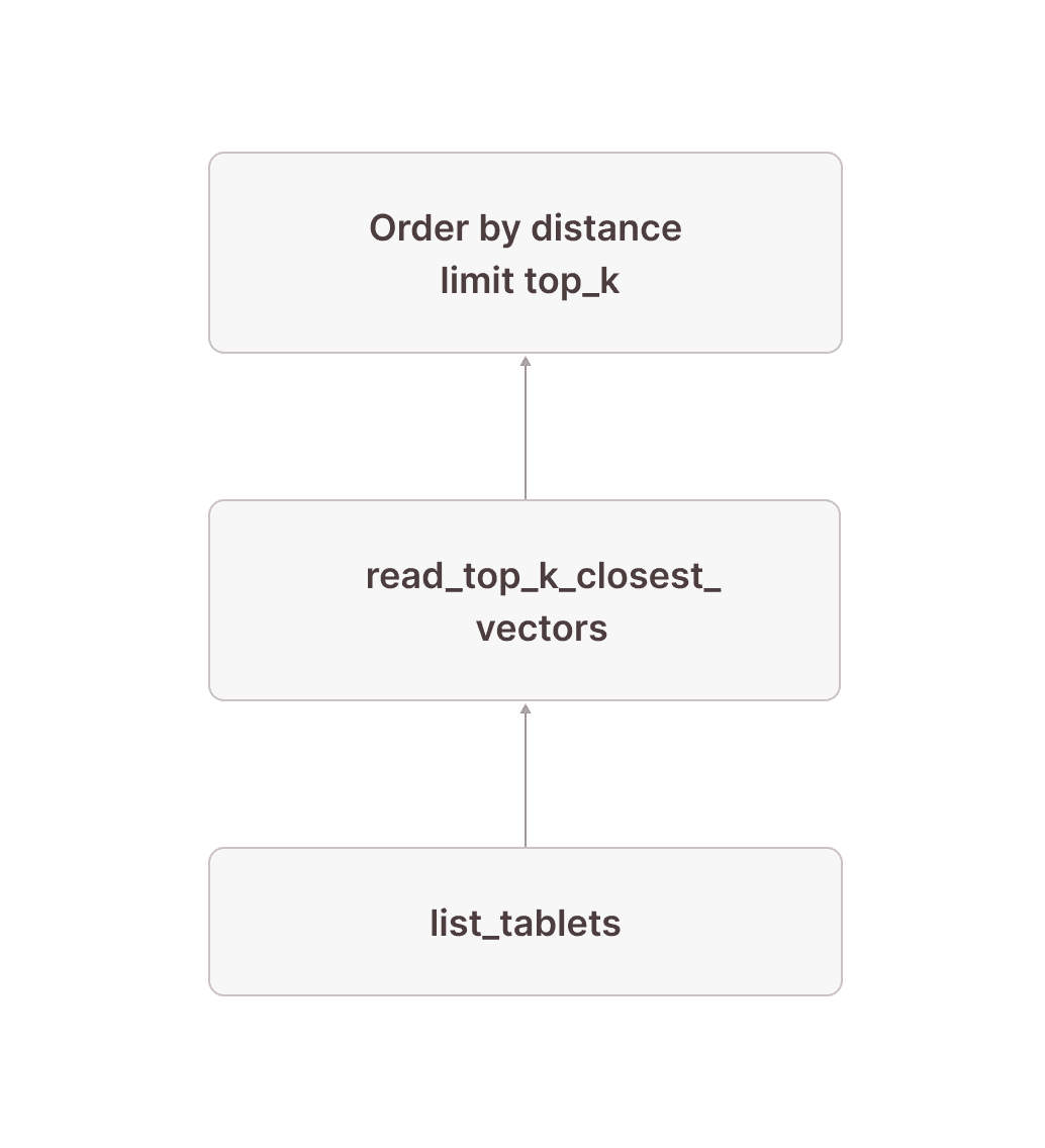
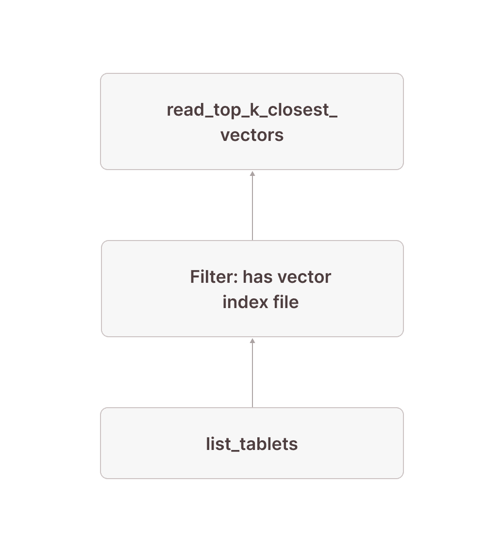
Let’s first look at a simplified version of the sub-plan of how we get tablet-id and the row numbers for the top 10 closest vectors to our target vector (we have removed some parts that will become important later). It is generally a good idea to read these query plans in the way data flows through them: From bottom to top. 

[12] [Sort] OrderBy: [read_top_k_closest_vectors.distance Ascending Last] Limit: [10]
 \_[13] [TableFuncScan] read_top_k_closest_vectors.tablet_id: $0.tablet_id, read_top_k_closest_vectors.tablet_row_number: $0.tablet_row_number, read_top_k_closest_vectors.distance: $0.distance
   |   $0 = read_top_k_closest_vectors(index => documents_vec_index, target_vector => target_vector, top_k => 10, ef_search => 64, load_strategy => in_memory, tablets => tablet)
   |   [Types]: read_top_k_closest_vectors.tablet_id: text not null, read_top_k_closest_vectors.tablet_row_number: bigint not null, read_top_k_closest_vectors.distance: double precision not null
    \_[14] [Projection] tablet, target_vector: ARRAY <target_vector>
      |   [Types]: target_vector: array(double precision not null) null
       \_[15] ...
          \_[16] ...
             \_[17] [TableFuncScan] tablet: $0.tablet
                   $0 = list_tablets(table_name => documents)
                   [Types]: tablet: tablet not null

We start in node [17] by listing all the tablets that are part of the documents table. After doing some things that will become important later, we add the target vector using a projection in node [14] (if the target vector is not a constant value, this might be replaced by a cross join with the subquery computing the target vector). Node [13] does the actual work: It is a TableFuncScan using the read_top_k_closest_vectors table-valued function (TVF). The read_top_k_closest_vectors TVF is an internal function that takes tablets and a target vector as input, reads the physical index files for each tablet, and searches them by the target vector. As output, we get up to top_k rows for each tablet with columns tablet_id and tablet_row_number to identify the rows in the base table, as well as distance, which is the distance of the corresponding vector in the table to the target vector. This distance is then used in node [12] to distill the top_k rows per tablet down to the overall top_k rows by ordering by the distance and keeping only the top_k closest rows. Conceptually, our plan now looks like this:

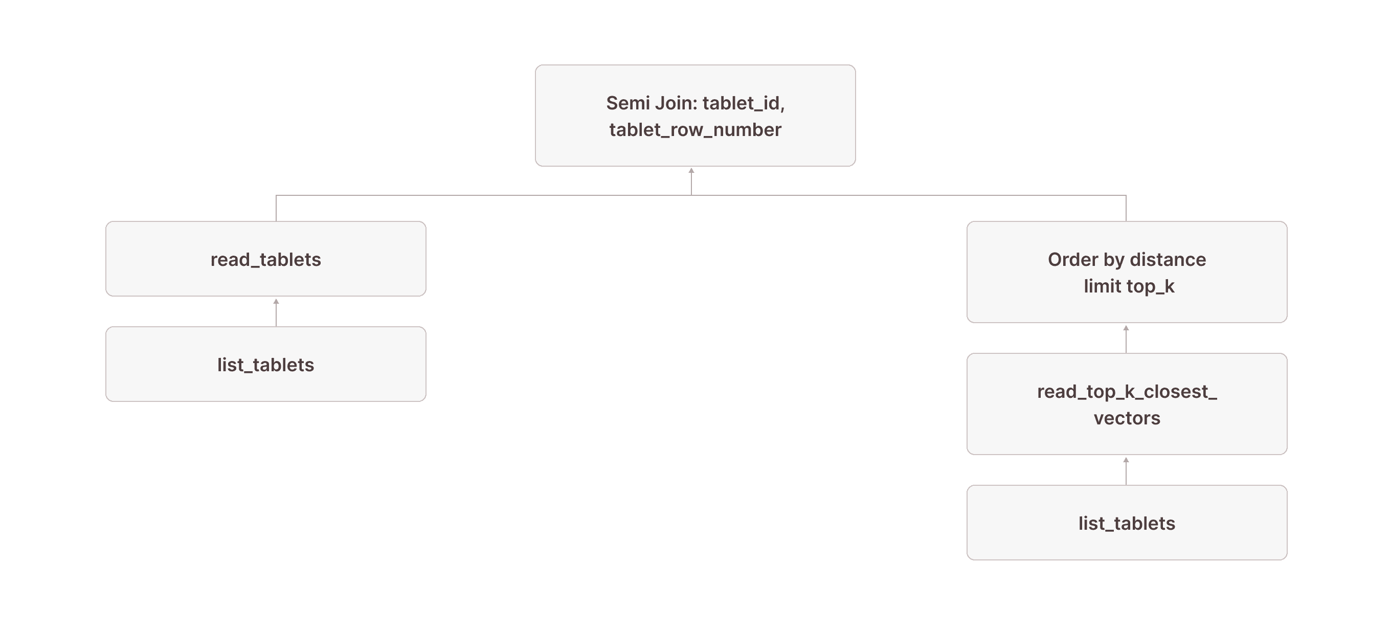
Next, we need to read the corresponding rows from the actual table:

[5] [Join] Mode: Semi [(tuple_0 = tuple_1)]
 \_[6] [Projection] documents.id, documents.embedding, documents.$tablet_id, documents.$tablet_row_number, tuple_0: tuple(documents.$tablet_id, documents.$tablet_row_number)
 | |   [Types]: tuple_0: tuple(text not null, bigint not null) not null
 |  \_[7] [TableFuncScan] documents.id: $0.id, documents.embedding: $0.embedding, documents.$tablet_id: $0.$tablet_id, documents.$tablet_row_number: $0.$tablet_row_number
 |    |   $0 = read_tablets(table_name => documents, tablet, tuple(documents.$tablet_id, documents.$tablet_row_number) in (SUBQUERY{0}))
 |    |   [Types]: documents.id: integer null, documents.embedding: array(real not null) not null, documents.$tablet_id: text not null, documents.$tablet_row_number: bigint not null
 |     \_[8] [TableFuncScan] tablet: $0.tablet
 |           $0 = list_tablets(table_name => documents)
 |           [Types]: tablet: tablet not null
 \_[9] ...
    \_[10] ...
       \_[11] [Projection] tuple_1: tuple(read_top_k_closest_vectors.tablet_id, read_top_k_closest_vectors.tablet_row_number)
         |   [Types]: tuple_1: tuple(text not null, bigint not null) not null
          \_[12] [Sort] OrderBy: [read_top_k_closest_vectors.distance Ascending Last, read_top_k_closest_vectors.tablet_id Ascending Last, read_top_k_closest_vectors.tablet_row_number Ascending Last] Limit: [10]

We continue with the same node [12] from above, which returns the tablet_id and tablet_row_number of the rows we want to read. In node [5], this result is used as the right side of a left semi-join, where the left side is a table scan of the documents table (nodes [7] and [8] are how table scans are represented in Firebolt's physical query plans). The join condition requires that the $tablet_id and $tablet_row_number from the documents table equal the values returned by the read_top_k_closest_vectors TVF. (The fact that this is modeled as a tuple in nodes [11] and [6] is an implementation detail that might change in the future.)

With this plan, we now have access to all columns of the base table for the exact rows returned by the vector search index:

Very observant readers might have noticed the in (SUBQUERY{0}) in node [7]. This is what allows us to scan only the rows returned by the read_top_k_closest_vectors TVF: we pass the result of node [9] (which contains the tablet_id and tablet_row_number columns) into the scan and use it for pruning. In the literature, this technique is often called sideways information passing or semi-join reduction:

SUBQUERY{0}:
[23] ... 
 \_[24] [Projection] tuple_1
    \_Recurring Node --> [9]

Our visualized plan now looks like this:

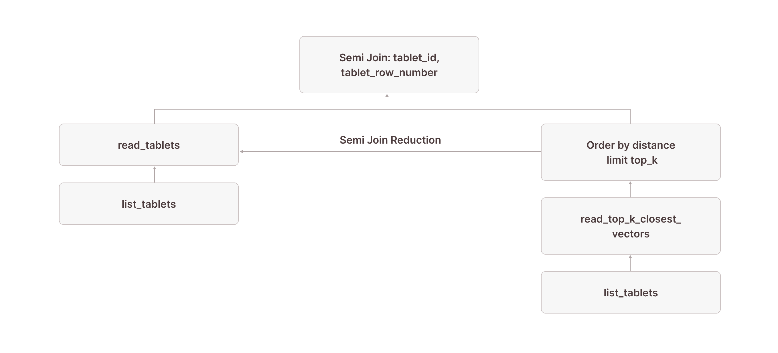
Because of this optimization, you would see something like granules: 10/1000000 for read_tablets in node [7] in the output of EXPLAIN(ANALYZE). This means that out of 1,000,000 granules in the table, only 10 were actually scanned—all thanks to read_top_k_closest_vectors doing the heavy lifting and semi-join reduction allowing us to prune the actual table scan.

This covers the core of how vector index queries are evaluated in Firebolt: we use the read_top_k_closest_vectors TVF and a [Sort] OrderBy: [distance] Limit: [10] operator to obtain the tablet IDs and row numbers of the 10 closest vectors to the target vector. We then use a semi-join with semi-join reduction to selectively scan the actual rows from the base table.

What About the Rest? Getting Results From Unindexed Tablets

But looking at the query plan, there is more going on. This is because Firebolt might produce tablets that don’t have vector index files. This could either be because the index was created on an already populated table without triggering index recreation or because Firebolt decided that a tablet is too small to be worth indexing. To see how this is handled, let’s look at nodes [15] and [16] that we left out before:

[13] [TableFuncScan] read_top_k_closest_vectors.tablet_id: $0.tablet_id, read_top_k_closest_vectors.tablet_row_number: $0.tablet_row_number, read_top_k_closest_vectors.distance: $0.distance
|   $0 = read_top_k_closest_vectors(index => documents_vec_index, target_vector => target_vector, top_k => 10, ef_search => 64, load_strategy => in_memory, tablets => tablet)
|   [Types]: read_top_k_closest_vectors.tablet_id: text not null, read_top_k_closest_vectors.tablet_row_number: bigint not null, read_top_k_closest_vectors.distance: double precision not null
 \_[14] [Projection] tablet, target_vector: ARRAY <target_vector>
   |   [Types]: target_vector: array(double precision not null) null
    \_[15] [Filter] contains(vector_search_index_files_in_tablet, 'documents_vec_index_547a5e0e_5bd0_4c98_8ec8_0874b248d511')
       \_[16] [Projection] tablet, vector_search_index_files_in_tablet: json_pointer_extract_keys(vector_search_index_sizes, '')
         |   [Types]: vector_search_index_files_in_tablet: array(text not null) null
          \_[17] [TableFuncScan] tablet: $0.tablet, vector_search_index_sizes: $0.vector_search_index_sizes
                $0 = list_tablets(table_name => documents)
                [Types]: tablet: tablet not null, vector_search_index_sizes: text null

Instead of just the tablets, we also retrieve the list of all vector index files (as well as their sizes) for each tablet from list_tablets in node [17]. Because this column is a JSON object, we use the json_pointer_extract_keys function in node [16] to extract an array containing the names of all vector search indexes that have a file for the given tablet and then in node [15] filter out any tablet that doesn’t have a file for the vector index documents_vec_index_547a5e0e_5bd0_4c98_8ec8_0874b248d51 which is the internal name Firebolt used for the documents_vec_index vector index. Note that we only need to perform this json operation once per tablet of which there are orders of magnitude fewer than rows in the table.

Conceptually, this is simply a filter that only keeps tablets that have a vector index file for the vector search index used in our query:

This means that everything we looked at in the previous section only obtains results from tablets that actually have a vector index file. We now need to make sure we also include rows from tablets without vector index files in the result.

The following subplan scans all tablets not covered by a vector index. The pattern is very similar to the one above, but this time we filter out any rows that do have a vector index file in node [20] and scan only the tablets that don't in node [18].

[18] [TableFuncScan] documents.id: $0.id, documents.embedding: $0.embedding, documents.$tablet_id: $0.$tablet_id, documents.$tablet_row_number: $0.$tablet_row_number
|   $0 = read_tablets(table_name => documents, tablet)
|   [Types]: documents.id: integer null, documents.embedding: array(real not null) not null, documents.$tablet_id: text not null, documents.$tablet_row_number: bigint not null
 \_[19] [Projection] tablet
    \_[20] [Filter] (not contains(vector_search_index_files_in_tablet, 'documents_vec_index_547a5e0e_5bd0_4c98_8ec8_0874b248d511'))
       \_[21] [Projection] tablet, vector_search_index_files_in_tablet: json_pointer_extract_keys(vector_search_index_sizes, '')
         |   [Types]: vector_search_index_files_in_tablet: array(text not null) null
          \_[22] [TableFuncScan] tablet: $0.tablet, vector_search_index_sizes: $0.vector_search_index_sizes
                $0 = list_tablets(table_name => documents)
                [Types]: tablet: tablet not null, vector_search_index_sizes: text null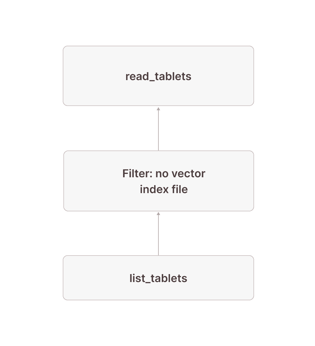

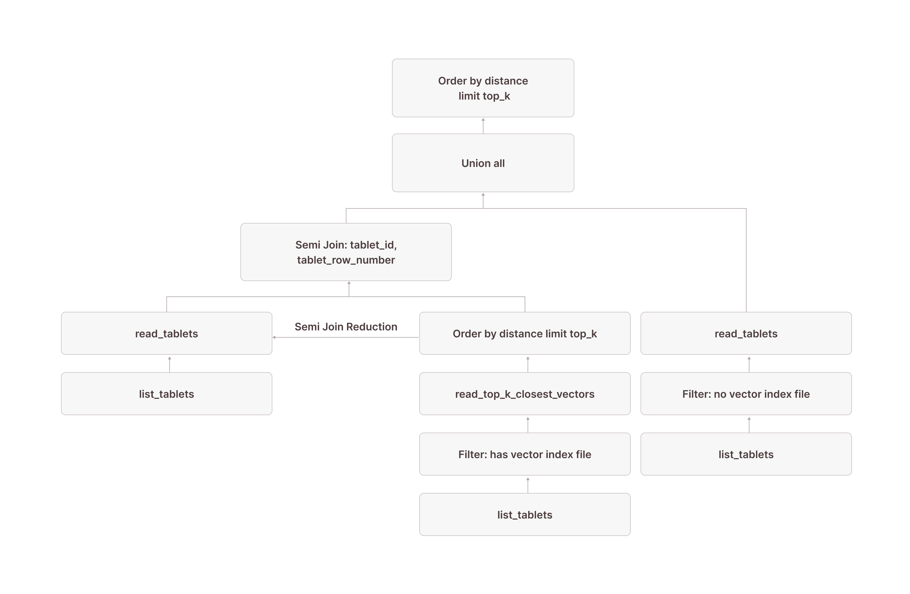
After this, we have all rows from tablets without vector index files after node [18] as well as up to 10 (the top_k parameter we used in the vector_search TVF) results from tablets with vector index files after the join in node [5]. We now need to retrieve the overall result from these two:

[0] [Projection] documents.id, documents.embedding
 \_[1] [Sort] OrderBy: [distance_to_target Ascending Last, documents.$tablet_id Ascending Last, documents.$tablet_row_number Ascending Last] Offset: [0] Limit: [10]
    \_[2] [Projection] documents.id, documents.embedding, documents.$tablet_id, documents.$tablet_row_number, distance_to_target: vector_cosine_distance(cast(documents.embedding as array(double precision)), ARRAY <target_vector>)
      |   [Types]: distance_to_target: double precision null
       \_[3] [Union]

Node [3] combines the results of nodes [5] and [18]. In node [2], we calculate the distance of each scanned row to the target vector using the vector_cosine_distance function (because the documents_vec_index index was created with the vector_cosine_ops operation). In node [1], we order by this distance and keep only the top 10 overall results. Finally, node [0] projects only the columns selected in the query (i.e., all columns of the documents table).

Putting it all together, this is what the complete query plan looks like:

[0] [Projection] documents.id, documents.embedding
 \_[1] [Sort] OrderBy: [distance_to_target Ascending Last, documents.$tablet_id Ascending Last, documents.$tablet_row_number Ascending Last] Offset: [0] Limit: [10]
    \_[2] [Projection] documents.id, documents.embedding, documents.$tablet_id, documents.$tablet_row_number, distance_to_target: vector_cosine_distance(cast(documents.embedding as array(double precision)), ARRAY <target_vector>)
      |   [Types]: distance_to_target: double precision null
       \_[3] [Union]
          \_[4] [Projection] documents.id, documents.embedding, documents.$tablet_id, documents.$tablet_row_number
          |  \_[5] [Join] Mode: Semi [(tuple_0 = tuple_1)]
          |     \_[6] [Projection] documents.id, documents.embedding, documents.$tablet_id, documents.$tablet_row_number, tuple_0: tuple(documents.$tablet_id, documents.$tablet_row_number)
          |     | |   [Types]: tuple_0: tuple(text not null, bigint not null) not null
          |     |  \_[7] [TableFuncScan] documents.id: $0.id, documents.embedding: $0.embedding, documents.$tablet_id: $0.$tablet_id, documents.$tablet_row_number: $0.$tablet_row_number
          |     |    |   $0 = read_tablets(table_name => documents, tablet, tuple(documents.$tablet_id, documents.$tablet_row_number) in (SUBQUERY{0}))
          |     |    |   [Types]: documents.id: integer null, documents.embedding: array(real not null) not null, documents.$tablet_id: text not null, documents.$tablet_row_number: bigint not null
          |     |     \_[8] [TableFuncScan] tablet: $0.tablet
          |     |           $0 = list_tablets(table_name => documents)
          |     |           [Types]: tablet: tablet not null
          |     \_[9] [Shuffle] Loopback with disjoint readers
          |       |   [Affinity]: single node
          |        \_[10] [Aggregate partial] GroupBy: [tuple_1] Aggregates: []
          |           \_[11] [Projection] tuple_1: tuple(read_top_k_closest_vectors.tablet_id, read_top_k_closest_vectors.tablet_row_number)
          |             |   [Types]: tuple_1: tuple(text not null, bigint not null) not null
          |              \_[12] [Sort] OrderBy: [read_top_k_closest_vectors.distance Ascending Last, read_top_k_closest_vectors.tablet_id Ascending Last, read_top_k_closest_vectors.tablet_row_number Ascending Last] Limit: [10]
          |                 \_[13] [TableFuncScan] read_top_k_closest_vectors.tablet_id: $0.tablet_id, read_top_k_closest_vectors.tablet_row_number: $0.tablet_row_number, read_top_k_closest_vectors.distance: $0.distance
          |                   |   $0 = read_top_k_closest_vectors(index => documents_vec_index, target_vector => target_vector, top_k => 10, ef_search => 64, load_strategy => in_memory, tablets => tablet)
          |                   |   [Types]: read_top_k_closest_vectors.tablet_id: text not null, read_top_k_closest_vectors.tablet_row_number: bigint not null, read_top_k_closest_vectors.distance: double precision not null
          |                    \_[14] [Projection] tablet, target_vector: ARRAY <target_vector>
          |                      |   [Types]: target_vector: array(double precision not null) null
          |                       \_[15] [Filter] contains(vector_search_index_files_in_tablet, 'documents_vec_index_547a5e0e_5bd0_4c98_8ec8_0874b248d511')
          |                          \_[16] [Projection] tablet, vector_search_index_files_in_tablet: json_pointer_extract_keys(vector_search_index_sizes, '')
          |                            |   [Types]: vector_search_index_files_in_tablet: array(text not null) null
          |                             \_[17] [TableFuncScan] tablet: $0.tablet, vector_search_index_sizes: $0.vector_search_index_sizes
          |                                   $0 = list_tablets(table_name => documents)
          |                                   [Types]: tablet: tablet not null, vector_search_index_sizes: text null
          \_[18] [TableFuncScan] documents.id: $0.id, documents.embedding: $0.embedding, documents.$tablet_id: $0.$tablet_id, documents.$tablet_row_number: $0.$tablet_row_number
            |   $0 = read_tablets(table_name => documents, tablet)
            |   [Types]: documents.id: integer null, documents.embedding: array(real not null) not null, documents.$tablet_id: text not null, documents.$tablet_row_number: bigint not null
             \_[19] [Projection] tablet
                \_[20] [Filter] (not contains(vector_search_index_files_in_tablet, 'documents_vec_index_547a5e0e_5bd0_4c98_8ec8_0874b248d511'))
                   \_[21] [Projection] tablet, vector_search_index_files_in_tablet: json_pointer_extract_keys(vector_search_index_sizes, '')
                     |   [Types]: vector_search_index_files_in_tablet: array(text not null) null
                      \_[22] [TableFuncScan] tablet: $0.tablet, vector_search_index_sizes: $0.vector_search_index_sizes
                            $0 = list_tablets(table_name => documents)
                            [Types]: tablet: tablet not null, vector_search_index_sizes: text null

SUBQUERY{0}:
[23] [AggregateState] GroupBy: [] Aggregates: [make_pruning_set_0: make_pruning_set(tuple_1, 5000000)]
|   [Types]: make_pruning_set_0: aggregatefunction(make_pruning_set(5000000), tuple(text not null, bigint not null) not null) not null
 \_[24] [Projection] tuple_1
    \_Recurring Node --> [9]

Or, using our simplified visualization:

Benchmarks

To evaluate the performance of our vector index under a realistic load, we ran a sustained workload against the unchanged production dataset from one of our customers who uses Firebolt’s vector index already in production on the same data.

Setup

The base table’s size is 1.64TiB (compressed) and consists of 435,488,243 embeddings of dimension 1024.

CREATE TABLE embeddings (
	id TEXT NOT NULL,
	embedding ARRAY(REAL NOT NULL) NOT NUL
) PRIMARY INDEX id;

The vector search index on this table is 691GiB in size.

CREATE INDEX embeddings_vec_index
ON embeddings
USING hnsw (embedding vector_cosine_ops)
WITH
	dimension=1024
	quantization='i8'
	connectivity=16 --default
	ef_consutrction=128 --default
;

The engine we used was an 8-node, single-cluster, storage-optimized (SO) one in the AWS region us-east-1. This engine configuration was chosen regarding its capability of caching the whole index, which is required for optimal performance (the vector index cache size limit was increased.

CREATE ENGINE <name>
WITH 
	nodes=8
	clusters=1
	family=SO
	type=M
	-- 75% of the engine's memory can be used for caching vector index
	vector_index_cache_memory_fraction=0.75
	-- 5% of the engine's memory can be used for caching query (sub-)results
	query_cache_memory_fraction=0.05
;

As a client, we used an EC2 instance in the same region to minimize network overhead.

Result

To evaluate our index, we look at two important metrics: latency at QPS and recall. We did not tune the index for any of these metrics and used the parameters’ default values. Furthermore, the build time of the index and warming up the engine are not part of the presented numbers. Before we ran the simulation, we warmed up the engine to ensure (1) all base table data is cached on the engine’s SSD and (2) the vector index is fully loaded into the engine’s memory

For measuring latency at QPS, we selected 10,000 random embeddings from the base table as target vectors and simulated a steady, multi-user workload. We simulated 3000 users, where each one executes a vector search query and then waits [1, 30] seconds before sending the next query.

We purposely disabled result caching to simulate a real-world use case where each target vector originates from an embedding model, which makes it likely unique and therefore unusable for result-reusage anyway.

SELECT keyword from vector_search (
	INDEX embeddings_vec_index,
	target_vector => <random selected embedding>, 
	top_k => 10,
	ef_search => 16 -- default value
) with (enable_subresult_cache = false);

At 3000 users with thinking time, we plateaued at a client-side-measured QPS of 190-200 with a p99 latency of 390ms (no query failures occurred). These numbers are measured on the client-side and therefore contain: HTTP request/response, (potential) query queueing, and query processing latency.

• p50: 170ms
• p60: 180ms
• P70: 200ms
• p80: 220ms
• p90: 260ms
• p95: 290ms
• p99: 390ms

Running this kind of concurrent workload without the index is not possible. On the same engine, a vector search without the index (single user, without any other queries running on the system) takes 80-90 seconds, while the search via the index is 1000-fold faster at 80ms.

The same (untuned) index achieved a recall@10 of 87% (measured across 1500 different, randomly selected target vectors). 

Cost

Firebolt’s concept of compute-storage separation allows us to calculate the exact cost for this benchmark. Therefore, we simply have to add up the S3 storage cost with the compute cost for every minute the engine is up and running.

• Base table with full precision data vectors: 1.64TiB ~= $41.47 / month
• Index with quantized data vectors: 691GiB ~= $17.06 / month
• Engine: 8M SO $44.80 / hour

Firebolt also supports running large indexes on much smaller engines without the need to load them into memory fully. This option is available as a parameter directly in the TVF itself with `load_strategy=’disk’`. We’ll try to keep as much as possible in memory on a best-effort basis. Through parallel load on the engine, memory and cache eviction can happen, which will cause unpredictable latency for this strategy, though.

SELECT keyword from vector_search (
	INDEX embeddings_vec_index,
	target_vector => <random selected embedding>, 
	top_k => 10,
	ef_search => 16,
	load_strategy => 'disk'
) with (enable_subresult_cache = false);

Wrapping Up: Vector Search in Firebolt

With vector search indexes, Firebolt makes it possible to run low-latency, high-throughput semantic search directly inside your data warehouse — without maintaining separate vector databases or compromising on ACID guarantees. By combining HNSW indexes with Firebolt’s tablet-based storage and execution engine, we can search hundreds of millions of high-dimensional embeddings in milliseconds, while staying fully transactional and tightly integrated with SQL.

In this post, we explored the architectural building blocks behind Firebolt’s vector search: how indexes are built and cached, how transactional consistency is maintained, and how query execution plans make use of these indexes to deliver fast top-K searches. We also covered best practices for engine sizing, index tuning, and table design to help you get the best performance for your workloads.

If you’re building semantic search, retrieval-augmented generation (RAG), or other AI-powered applications, Firebolt’s native vector search capabilities let you keep your data and your queries in one place, fast, reliable, and SQL-native.

Start using Firebolt’s vector search indexes today:

• Explore the Firebolt documentation (coming soon) to learn more about CREATE INDEX, vector_search, and tuning parameters.

Try out your own workloads with vector search indexes to see how far you can push performance with $200 in free credits to get you started.