In this blog post you will learn how GROUPING SETS work and how Firebolt’s implementation uses smart query planning to execute them efficiently.

Introduction - What GROUPING SETS do for you

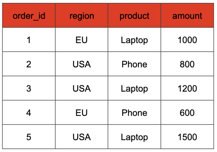
When working with SQL queries, reporting and analytics often require summarizing the same data in multiple different ways. Let’s say we have the following table tracking orders of our products:

We might be interested in multiple aggregations here:

1. the total sales amount per region and product
2. the total sales amount per region
3. the total sales amount over all orders.

‍

Usually we would cover any of these points with a GROUP BY statement. For example, to get the total sales amount per region and product we would query the data with

SELECT 
    region, product, SUM(amount) AS total_sales 
FROM
    orders 
GROUP BY
    region, product;

‍

But how do we get all three aggregations in our query? Instead of writing multiple GROUP BY statements, SQL provides a powerful feature called GROUPING SETS, which allows for multiple aggregations in one go:

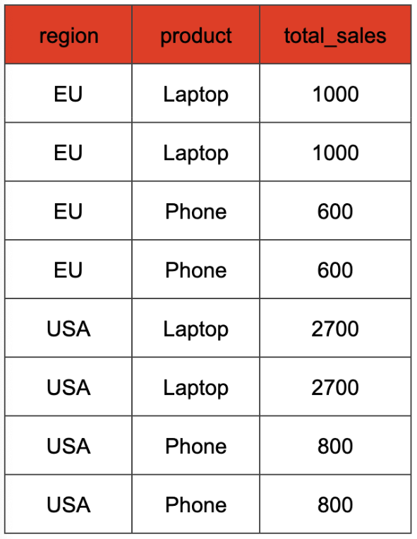
SELECT
    region, product, SUM(sales_amount) AS total_sales 
FROM
    orders 
GROUP BY GROUPING SETS ( 
    (region, product), -- Sales per region and product 
    (region),          -- Sales per region
    ()                 -- Grand total sales 
);

With this query, the result table will look something like this:

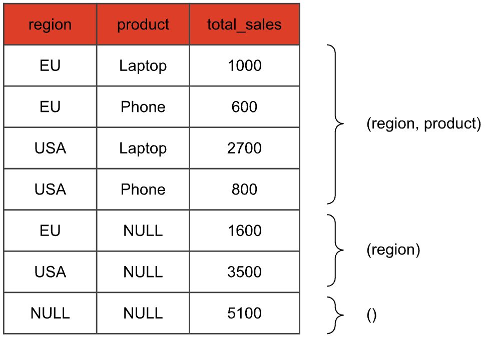
We just did three aggregations in one swoop: The first four rows are the result of the aggregation with both region and product, the next two rows aggregate only by the region, and the last row corresponds to the empty grouping set (also called grand total), that evaluates the aggregate function without a GROUP BY key. Columns that are not part of the grouping set of the current aggregation are set to NULL.

Rewriting GROUPING SETS

So we have seen that GROUPING SETS can be used to request the same aggregates for different sets of grouping keys in a concise way. Imagine you were confronted with a SQL database that does not support GROUPING SETS syntax. The first idea you might have is to write a query like this: 

SELECT region, product, SUM(amount) AS total_sales
FROM orders
GROUP BY region, product

UNION ALL

SELECT region, NULL, SUM(amount) AS total_sales
FROM orders
GROUP BY region

UNION ALL

SELECT NULL, NULL, SUM(amount) AS total_sales
FROM orders

‍

The output would be the same, but the query is much more verbose. But maybe one could implement GROUPING SETS this way? Just rewrite any statement containing GROUPING SETS into one that the runtime can already execute. The GROUPING SETS would only exist at the query planner level and would internally be transformed.

But using UNION ALL for this is probably not a good idea. We want to have as few scans over the base table as possible so we only have to read it in once. With this approach however we would have one scan per grouping set. That corresponds to the FROM orders part of the query. The amount of scans over our base table therefore increases linearly with the amount of grouping sets we have. This gets even worse when you calculate your grouping set over more than just a base table. Imagine you compute grouping sets on the result of joining terabytes of data. The UNION ALL strategy would mean that you need to evaluate that very expensive join once for each grouping set.

But there is a smarter way of rewriting a query with GROUPING SETS. Let’s take a look:

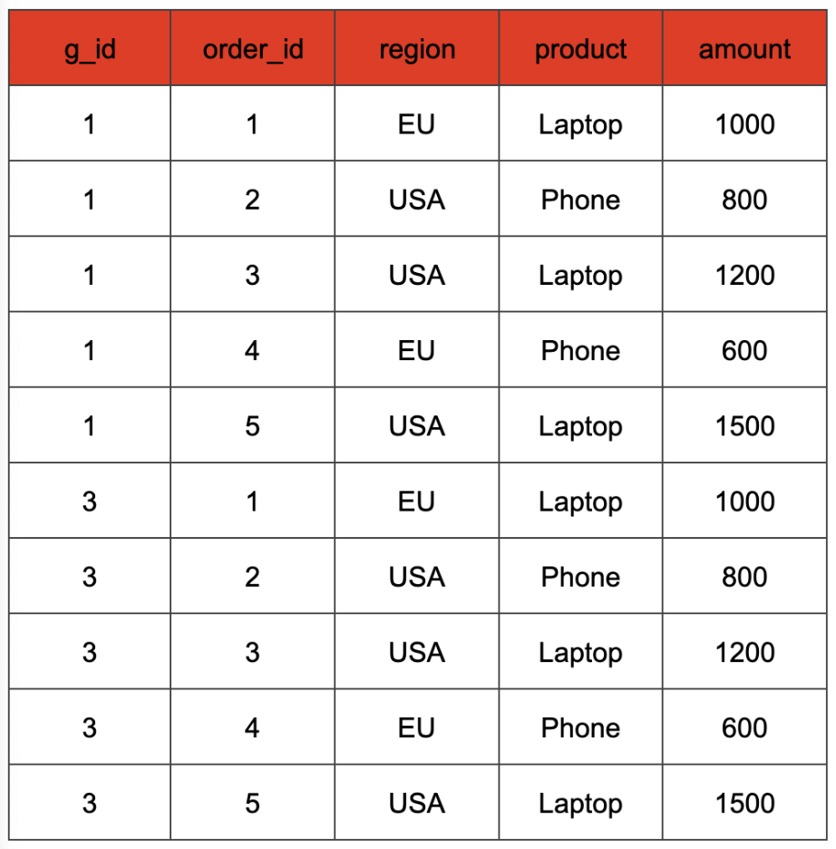
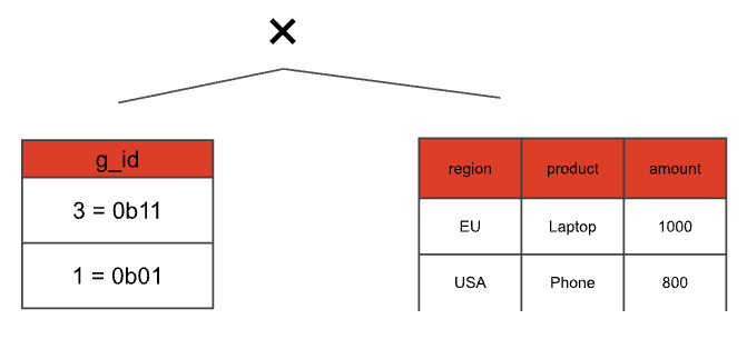
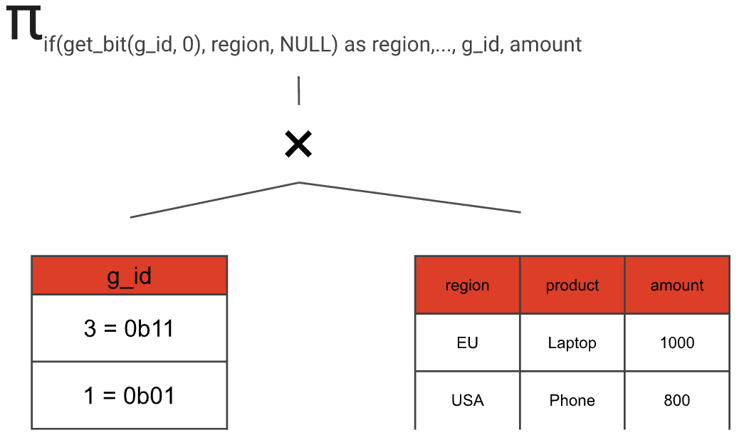
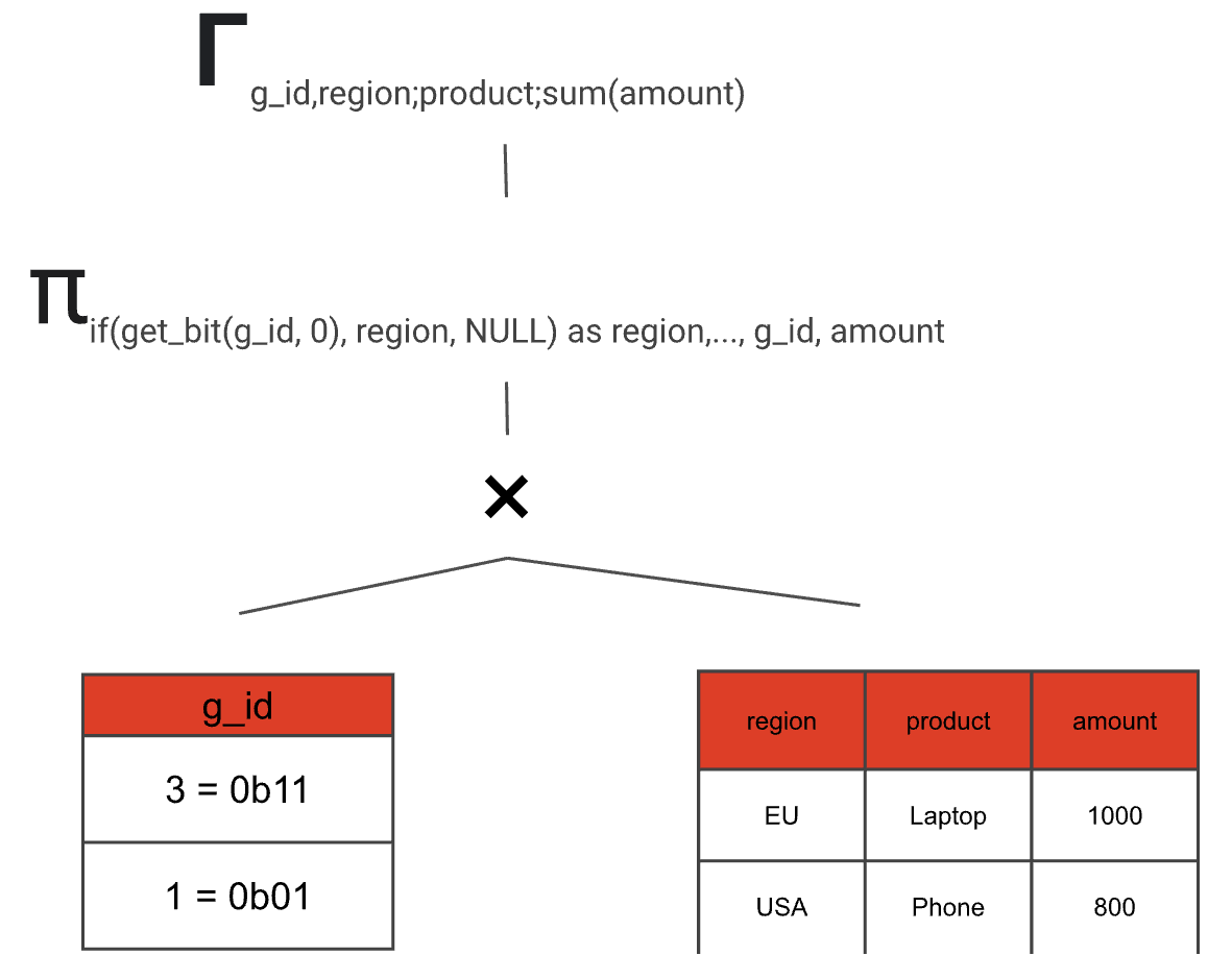
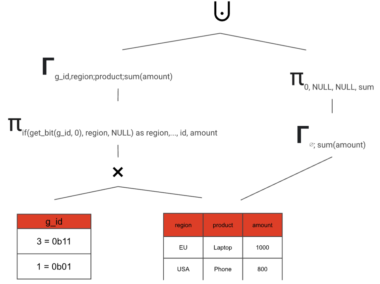
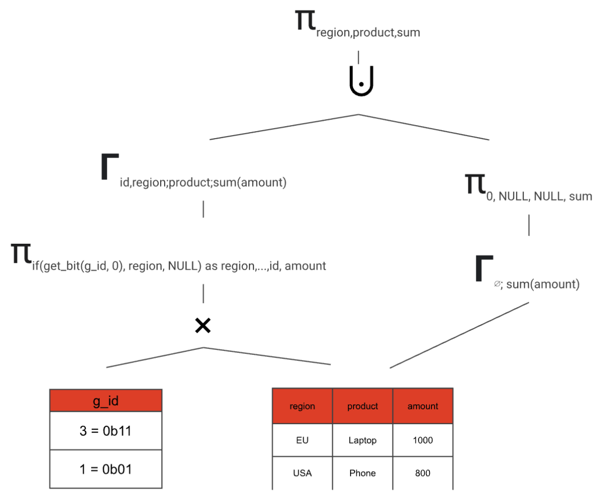
SELECT
    case when get_bit(gs.id, 0)
        then region
        else NULL end as region,
    case when get_bit(gs.id, 1)
        then product
        else NULL end as product,
    SUM(amount)
FROM
    orders,
    UNNEST(ARRAY[3, 1]) as grouping_sets(g_id)
GROUP BY
    grouping_id, 1, 2

UNION ALL

SELECT 
    NULL as region,
    NULL as product,
    SUM(amount)
FROM
    orders

‍

What happens here? Let’s focus on the first SELECT for now. In the FROM clause, we not only scan our base table, but also construct a cross join with a static table grouping_sets that contains a single g_id column that encodes the columns participating in the requested grouping set. Each input tuple from table orders is paired with each g_id value. Our example table after this cross join would look like this:

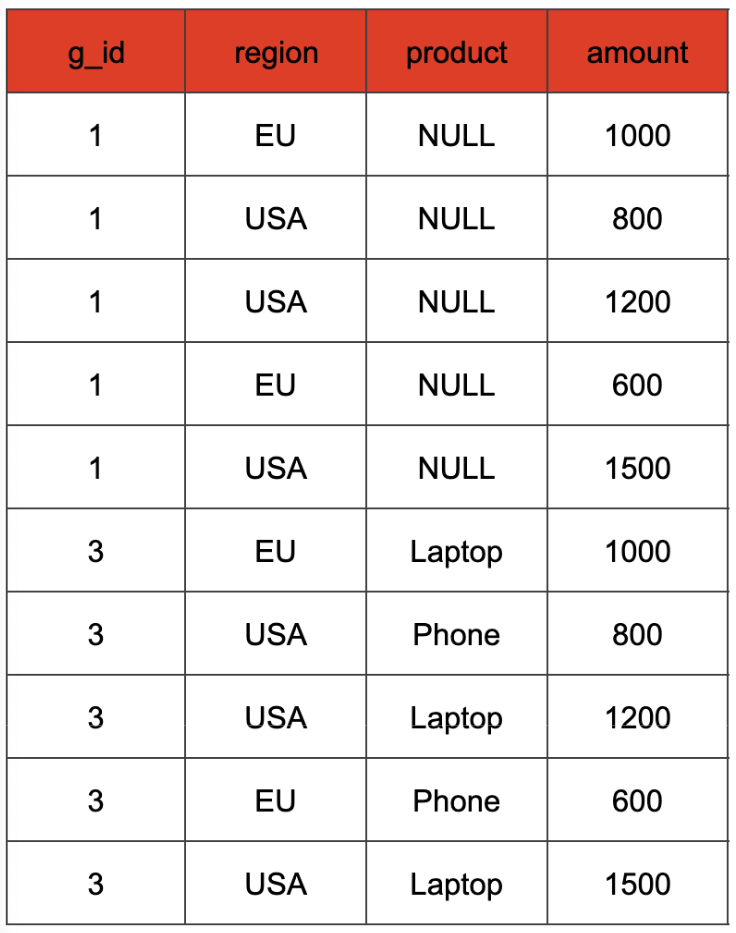
The values of the g_id column represent a binary encoding of the different combinations of the expressions passed as arguments to the GROUPING SETS clause. In our case, the two columns used in the GROUP BY clause are “region” and “product”. Hence, we have two binary positions that can either be set to 1, if the column is used in the grouping set, or to 0 otherwise. This way, we can distinguish the different grouping sets and do a GROUP BY that covers all of them. For instance, in our example a g_id value of 3 (binary 0b11) denotes the grouping set that includes both columns, while a g_id value of 1 (binary 0b01) denotes the grouping set containing only the "region" column. Consequently, in the SELECT clause, we can retain the original column value if the corresponding g_id bit is 1, and map it to NULL if that bit is 0 (we can check this with the get_bit function). The aggregate input of the SELECT statement from our example query looks like that.

The GROUP BY clause uses the g_id and the possibly NULL-mapped region and product columns as the key.

The special case of an empty input requires grand totals to be handled separately. This is because a GROUP BY clause with an empty grouping key should return the default NULL value for each aggregate function, rather than an empty result.

What’s so great about this rewrite is that we can compute any amount of grouping sets with at most two scans and two aggregations. And by having one larger aggregation instead of multiple smaller ones we can take full advantage of Firebolt’s distributed aggregation computation.

How GROUPING SETS are transformed from start to finish

After the parsing stage, a GROUP BY clause that utilizes GROUPING SETS is internally represented as a special aggregation node within the query plan. This node stores all the information pertaining to the grouping sets by using bitsets, which function similarly to the g_id values in the rewritten SQL query.

This special node only exists at the beginning of the logical query plan. This logical plan is an abstract representation of our query that we can use to perform optimizations using rules. The rules run over the tree and try to find patterns that they can optimize. In our case we use a rule that matches on this special aggregation node and transforms it subtree implementing the rewrite strategy outlined as a SQL-level rewrite above. The resulting plan consists of nodes that can already be executed by our runtime, so no runtime extensions are needed for adding support for GROUPING SETS.

Let's examine what the rule does in detail.

1. Create the grouping_sets(g_id) static table and the cross join. We can just interpret the bitsets in our special aggregation node as integers and build a table this way.

2. Build a projection that optionally maps grouping set expressions to NULL depending on the current g_id value. In addition, the projection retains the g_id value and all aggregate input columns.

3. Add an aggregation node

4. Do the same thing, but for the grand total (if requested in the SQL query) and combine both paths

5. Remove the g_id with another projection

And just like this, we transformed our GROUPING SETS aggregate node into an equivalent logical plan that can be further optimized and later executed.

There is one more edge case that we need to cover in the query planner: duplicate GROUPING SETS. A query like

SELECT
    region,
    prodcut,
    SUM(amount) as total_sales
FROM 
    orders
GROUP BY
    GROUPING SETS ((region,product),(region,product))

‍

has the grouping set (region, product) repeated twice. This leads to the aggregation result being duplicated:

We want to compute the aggregation without the duplicates first, and then duplicate the rows later, when we already have the correct aggregation result. That means our cross join would look like this:

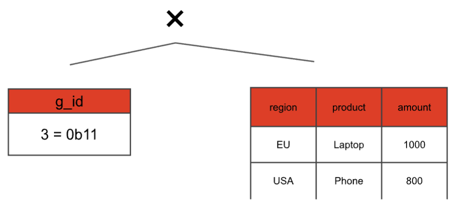
Even though we have two grouping sets that correspond to g_id = 3 we only have one 3 in the static table. We only consider the duplicates later, by adding another join on top with a static table that keeps the multiplicity:

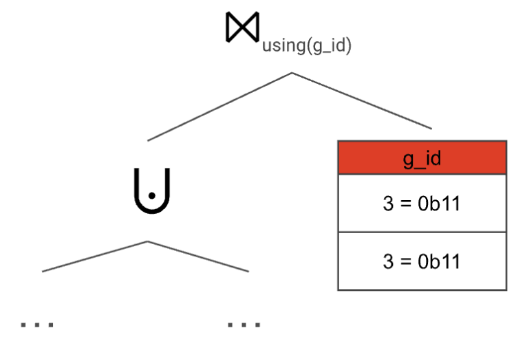
With this setup, we make sure to compute the GROUP BY both correctly and efficiently—no matter how often a grouping set appears in the GROUPING SETS clause, all aggregate functions are only computed once per distinctgrouping set.

‍

The grouping function

You might have noticed a problem with GROUPING SETS so far: The data might contain NULL values, so how do we differentiate between them and the NULL values added by the aggregation? SQL also offers a function for that, called grouping. Similar to our g_id, the function takes expressions found in any grouping set as arguments and produces an integer that represents each expression as a single bit. In this case, a 0 bit in the integer indicates that the expression is part of the aggregation.

If our initial query had utilized the grouping function:

SELECT 
    grouping(region, product) AS grouping, 
    region, product, 
    SUM(amount) AS total_sales
FROM
    orders
GROUP BY 
    GROUPING SETS ((region, product), region, ())

‍

The result would look like this:

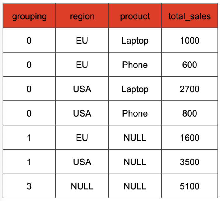
Grouping functions are also evaluated during planning—for each row the correct value is computed based on the current g_id value and the arguments of the grouping function call. The values can then later be joined and added to the result. 

Conclusion

GROUPING SETS offer a powerful way to perform multiple aggregations in a single SQL query, improving readability and conciseness. Firebolt's implementation leverages smart query planning to efficiently execute these aggregations by internally rewriting them. When transforming GROUPING SETS into a series of joins and aggregations, Firebolt minimizes table scans and optimizes distributed computation, ensuring high performance even with intricate grouping requirements.